Transforming Seasonal Challenges into Opportunities

If you’re in the home heating and services business, you’re familiar with the challenge of slow summers. While it’s a well-known phenomenon, as profit-seeking business owners, it makes sense to understand the situation rather than simply accept it as inevitable.

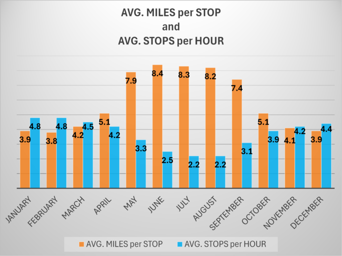
As the seasons progress from winter to spring and on into summer, our key metrics undergo noticeable shifts:

• • Degree-days diminish and then disappear impacting our delivery schedules
  • Reduced deliveries yield higher Stops/Hour drop and Miles/Stop
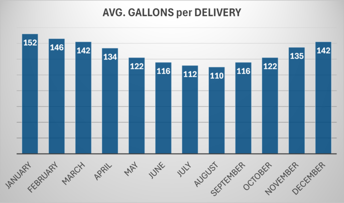
  • Average delivery sizes decrease

But why do average delivery sizes decrease?

We schedule deliveries based on tank capacity and customer consumption patterns. Even with fewer deliveries, I ask again, why are they smaller? The data tells us one possible cause could be discrepancies between reported tank levels and actual levels, often observed in non-monitored tanks.

Let’s review:

Tank levels (for unmonitored tanks) are calculated based on a starting level – when the tank is filled – and then the Back-office System (BOS) calculates consumption and “counts down” the in-tank levels (ITLs). The formula includes a combination of Baseload and K-factor consumption. This is where the trouble starts, especially in the shoulder months (leading up to and leaving the winter). Turns out that the BOS is not the culprit; customer behavior is.

Is the baseload correct? It’s hard to tell and there is no measurement to check non-heat usage. How many people are home in the spring and how much hot water do they use? As to the K-factor, while there are many theories for changing consumption patterns as it warms up, ultimately there is a linkage between the weather and consumption (unless someone shuts off their system for the summer). At that point, even if there are just a few HDDs on a given day the BOS will calculate consumption (based on the weather), but since the equipment is off, no heat-based consumption occurred. Lastly, many BOS have a set of seasonal Ks that usher in different consumption calculations based more on the calendar than the weather.

As you can see, there are many variables. You can surmise that consumption in the middle of the winter is more predictable than during the spring, summer and fall. You can even defend the case that as non-winter consumption is hard to predict, it would be reasonable to overestimate consumption – after all, a small delivery (caused by overstating consumption) is better than a run out any time of year.

Here’s the good news; while deliveries in the summer and fall are generally smaller than intended, the BOS (a proximate cause) can provide a solution. The data is right in front of you and just requires some analysis. If you break down your historical deliveries by customer and time of year, you can create a matrix, a treasure map of sorts, that can provide insights into which tanks are most and least likely to have small deliveries as well as how small those deliveries might be.

We call it the Lefty Shift and use that data to mitigate the issue for many of our clients, while being fully aware that the penalty for runouts is much harsher than the reward for larger deliveries.

Improving summer deliveries not only boosts revenue during off-peak periods but also streamlines operations during the crucial winter months allowing for more efficient winter deliveries and less overtime.

You could continue to simply make small summer deliveries, but that will cost you as your competitors become more efficient.

While small summer deliveries may seem inevitable, proactive analysis and strategic adjustments can transform seasonal challenges into opportunities for growth. Remember, the solutions lie within your data – they just need to be extracted and applied strategically.